Meshes.jl

Computational geometry and meshing algorithms in Julia.

Overview

Meshes.jl provides efficient implementations of concepts from computational geometry. It promotes rigorous mathematical definitions of spatial discretizations (a.k.a. meshes) that are adequate for describing general manifolds embedded in $\R^n$, including surfaces described with spherical coordinates, and geometries described with multiple coordinate reference systems.

Unlike other existing efforts in the Julia ecosystem, this project is being carefully designed to facilitate the use of meshes across different scientific domains. We follow a strict set of good software engineering practices, and are quite pedantic in our test suite to make sure that all our implementations are free of bugs in both single and double floating point precision. Additionally, we guarantee type stability.

The design of this project was motivated by various issues encountered with past attempts to represent geometry, which have been originally designed for visualization purposes (e.g. GeometryTypes.jl, GeometryBasics.jl) or specifically for finite element analysis (e.g. JuAFEM.jl, MeshCore.jl). We hope to provide a smoother experience with mesh representations that are adequate for finite finite element analysis, advanced geospatial modeling and visualization, not just one domain.

For advanced data science with geospatial data (i.e., tables over meshes), consider the GeoStats.jl framework. It provides sophisticated methods for estimating (interpolating), simulating and learning geospatial functions over Meshes.jl meshes. Please check the Geospatial Data Science with Julia book for more information:

If you have questions or would like to brainstorm ideas in general, don't hesitate to start a thread in our zulip channel. We are happy to improve the ecosystem to meet user's needs.

Installation

Get the latest stable release with Julia's package manager:

] add Meshes

Quick example

Although we didn't have time to document the functionality of the package properly, we still would like to illustrate some important features. For more information on available functionality, please consult the Reference guide and the suite of tests in the package.

In all examples we assume the following packages are loaded:

using Meshes
import CairoMakie as Mke

Points and vectors

A Point is defined by its coordinates in a global reference system. The type of the coordinates is determined automatically based on the specified literals, or is forced to a specific type using helper constructors (e.g. Point2, Point3, Point2f, Point3f). Integer coordinates are converted to Float64 to fulfill the requirements of most geometric processing algorithms, which would be undefined in a discrete scale.

A vector Vec follows the same pattern. It can be constructed with the generic Vec constructor or with the variants Vec2 and Vec3 for double precision and Vec2f and Vec3f for single precision.

# 2D points
A = Point(0.0, 1.0) # double precision as expected
B = Point(0f0, 1f0) # single precision as expected
C = Point(0, 0) # Integer is converted to Float64 by design
D = Point2(0, 1) # explicitly ask for double precision
E = Point2f(0, 1) # explicitly ask for single precision

# 3D points
F = Point(1.0, 2.0, 3.0) # double precision as expected
G = Point(1f0, 2f0, 3f0) # single precision as expected
H = Point(1, 2, 3) # Integer is converted to Float64 by design
I = Point3(1, 2, 3) # explicitly ask for double precision
J = Point3f(1, 2, 3) # explicitly ask for single precision

for P in (A,B,C,D,E,F,G,H,I,J)
  println("Coordinate type: ", coordtype(P))
  println("Embedding dimension: ", embeddim(P))
end

Coordinate type: Float64
Embedding dimension: 2
Coordinate type: Float32
Embedding dimension: 2
Coordinate type: Float64
Embedding dimension: 2
Coordinate type: Float64
Embedding dimension: 2
Coordinate type: Float32
Embedding dimension: 2
Coordinate type: Float64
Embedding dimension: 3
Coordinate type: Float32
Embedding dimension: 3
Coordinate type: Float64
Embedding dimension: 3
Coordinate type: Float64
Embedding dimension: 3
Coordinate type: Float32
Embedding dimension: 3

Points can be subtracted to produce a vector:

B - A

Vec(0.0, 0.0)

They can't be added, but their coordinates can:

coordinates(F) + coordinates(H)

Vec(2.0, 4.0, 6.0)

We can add a point to a vector though, and get a new point:

F + Vec(1, 1, 1)

Point(2.0, 3.0, 4.0)

And finally, we can create points at random with:

ps = rand(Point2, 10)

10-element Vector{Point2}:
 Point(0.10496224673370858, 0.9344071222047816)
 Point(0.05074868514695452, 0.339786347979961)
 Point(0.09768449815022762, 0.37474108542030493)
 Point(0.6378379548785978, 0.11746537316590555)
 Point(0.7970316403090639, 0.46560810798243646)
 Point(0.6502962468069529, 0.013212026720208936)
 Point(0.33205430358885524, 0.12065275259349528)
 Point(0.4091483160047814, 0.9910650013912135)
 Point(0.9353014989380538, 0.9303892040830068)
 Point(0.2829326427230989, 0.8804701360573512)

Primitives

Primitive geometries such as Box, Ball, Sphere, Cylinder are those geometries that can be efficiently represented in a computer without discretization. We can construct such geometries using clean syntax:

b = Box((0.0, 0.0, 0.0), (1.0, 1.0, 1.0))

viz(b)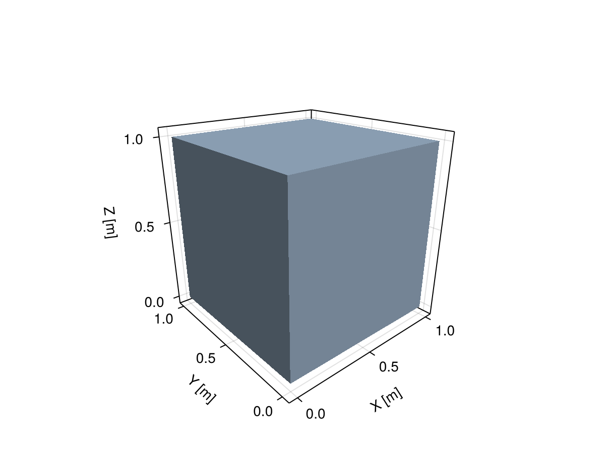

s = Sphere((0.0, 0.0, 0.0), 1.0)

viz(s)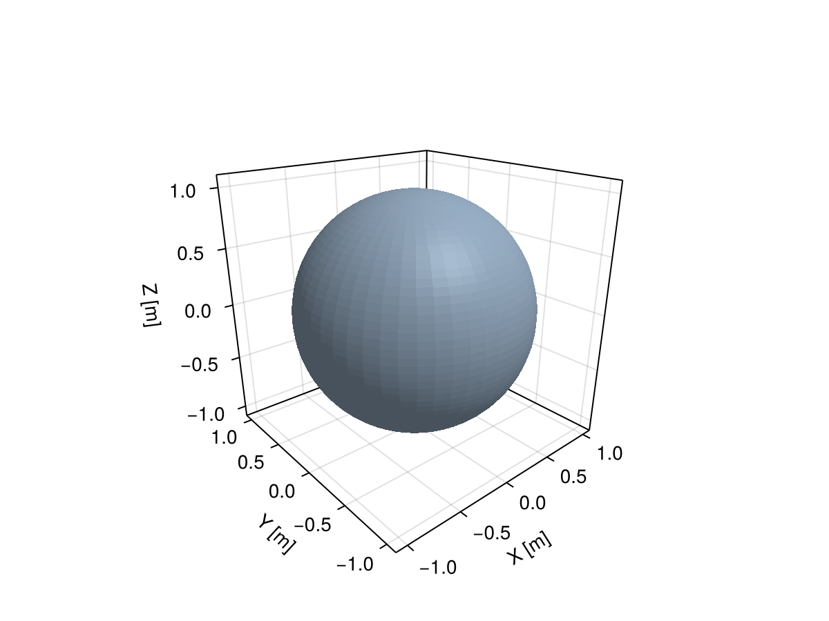

The parameters of these primitive geometries can be queried easily:

extrema(b)

(Point(0.0, 0.0, 0.0), Point(1.0, 1.0, 1.0))

centroid(s), radius(s)

(Point(0.0, 0.0, 0.0), 1.0)

As well as their measure (e.g. area, volume) and other geometric properties:

measure(b)

1.0

We can sample random points on primitives using different methods:

vs = sample(s, RegularSampling(10)) # 10 points over the sphere

Base.Iterators.Flatten{Base.Generator{Tuple{Base.Generator{Base.Iterators.ProductIterator{Tuple{StepRangeLen{Float64, Base.TwicePrecision{Float64}, Base.TwicePrecision{Float64}, Int64}, StepRangeLen{Float64, Base.TwicePrecision{Float64}, Base.TwicePrecision{Float64}, Int64}}}, Meshes.var"#350#354"{Sphere{3, Float64}}}, Base.Generator{Tuple{Point3, Point3}, typeof(identity)}}, typeof(identity)}}(Base.Generator{Tuple{Base.Generator{Base.Iterators.ProductIterator{Tuple{StepRangeLen{Float64, Base.TwicePrecision{Float64}, Base.TwicePrecision{Float64}, Int64}, StepRangeLen{Float64, Base.TwicePrecision{Float64}, Base.TwicePrecision{Float64}, Int64}}}, Meshes.var"#350#354"{Sphere{3, Float64}}}, Base.Generator{Tuple{Point3, Point3}, typeof(identity)}}, typeof(identity)}(identity, (Base.Generator{Base.Iterators.ProductIterator{Tuple{StepRangeLen{Float64, Base.TwicePrecision{Float64}, Base.TwicePrecision{Float64}, Int64}, StepRangeLen{Float64, Base.TwicePrecision{Float64}, Base.TwicePrecision{Float64}, Int64}}}, Meshes.var"#350#354"{Sphere{3, Float64}}}(Meshes.var"#350#354"{Sphere{3, Float64}}(Sphere(center: (0.0, 0.0, 0.0), radius: 1.0)), Base.Iterators.ProductIterator{Tuple{StepRangeLen{Float64, Base.TwicePrecision{Float64}, Base.TwicePrecision{Float64}, Int64}, StepRangeLen{Float64, Base.TwicePrecision{Float64}, Base.TwicePrecision{Float64}, Int64}}}((0.09090909090909091:0.09090909090909091:0.9090909090909091, 0.0:0.1:0.9))), Base.Generator{Tuple{Point3, Point3}, typeof(identity)}(identity, (Point(0.0, 0.0, 1.0), Point(0.0, 0.0, -1.0))))))

And collect the generator with:

viz(collect(vs))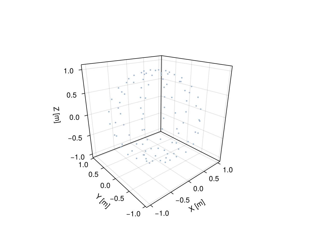

Polytopes

Polytopes are geometries with "flat" sides. They generalize polygons and polyhedra. Most commonly used polytopes are already defined in the project, including Segment, Ngon (e.g. Triangle, Quadrangle), Tetrahedron, Pyramid and Hexahedron.

t = Triangle((0.0, 0.0), (1.0, 0.0), (0.0, 1.0))

viz(t)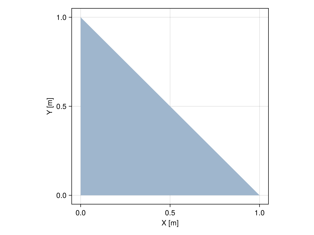

Some of these geometries have additional functionality like the measure (or area):

measure(t) == area(t) == 1/2

true

Or the ability to know whether or not a point is inside:

p = Point(0.5, 0.0)

p ∈ t

true

For line segments, for example, we have robust intersection algorithms:

s1 = Segment((0.0, 0.0), (1.0, 0.0))
s2 = Segment((0.5, 0.0), (2.0, 0.0))

s1 ∩ s2

Segment{2,Float64}
├─ Point(0.5, 0.0)
└─ Point(1.0, 0.0)

Polytopes are widely used in GIS software under names such as "LineString" and "Polygon". We provide robust implementations of these concepts, which are formally known as polygonal Chain and PolyArea.

We can compute the orientation of a chain as clockwise or counter-clockwise, can open and close the chain, create bridges between the various inner rings with the outer ring, and other useful functionality:

p = PolyArea((0,0), (2,0), (2,2), (1,3), (0,2))

viz(p)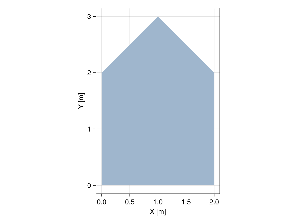

The orientation of the above polygonal area is counter-clockwise (CCW):

orientation(p)

CCW::OrientationType = 1

We can get the outer ring, and reverse it:

r = rings(p) |> first

reverse(r)

Ring{2,Float64}
├─ Point(0.0, 0.0)
├─ Point(0.0, 2.0)
├─ Point(1.0, 3.0)
├─ Point(2.0, 2.0)
└─ Point(2.0, 0.0)

A ring has circular vertices:

v = vertices(r)

5-element CircularVector(::Vector{Point2}):
 Point(0.0, 0.0)
 Point(2.0, 0.0)
 Point(2.0, 2.0)
 Point(1.0, 3.0)
 Point(0.0, 2.0)

This means that we can index the vertices with indices that go beyond the range 1:nvertices(r). This is very useful for writing algorithms:

v[1:10]

10-element CircularVector(::Vector{Point2}):
 Point(0.0, 0.0)
 Point(2.0, 0.0)
 Point(2.0, 2.0)
 Point(1.0, 3.0)
 Point(0.0, 2.0)
 Point(0.0, 0.0)
 Point(2.0, 0.0)
 Point(2.0, 2.0)
 Point(1.0, 3.0)
 Point(0.0, 2.0)

We can also compute angles of any given chain, no matter if it is open or closed:

angles(r) * 180 / pi

5-element Vector{Float64}:
  -90.0
  -90.0
 -135.0
  -90.0
 -135.0

The sign of these angles is a function of the orientation:

angles(reverse(r)) * 180 / pi

5-element Vector{Float64}:
  90.0
 135.0
  90.0
 135.0
  90.0

In case of rings (i.e. closed chains), we can compute inner angles as well:

innerangles(r) * 180 / pi

5-element Vector{Float64}:
  90.0
  90.0
 135.0
  90.0
 135.0

And there is a lot more functionality available like for instance determining whether or not a polygonal area or chain is simple:

issimple(p)

true

Meshes

Efficient (lazy) mesh representations are provided, including CartesianGrid and SimpleMesh, which are specific types of Domain:

Domain

grid = CartesianGrid(100, 100)

viz(grid, showsegments = true)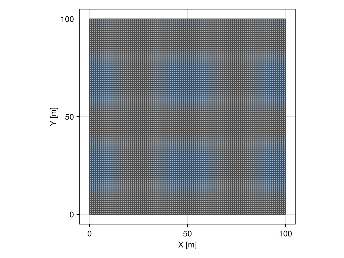

No memory is allocated:

@allocated CartesianGrid(10000, 10000, 10000)

0

but we can still loop over the elements, which are quadrangles in 2D:

collect(grid)

10000-element Vector{Quadrangle{2, Float64}}:
 Quadrangle((0.0, 0.0), ..., (0.0, 1.0))
 Quadrangle((1.0, 0.0), ..., (1.0, 1.0))
 Quadrangle((2.0, 0.0), ..., (2.0, 1.0))
 Quadrangle((3.0, 0.0), ..., (3.0, 1.0))
 Quadrangle((4.0, 0.0), ..., (4.0, 1.0))
 Quadrangle((5.0, 0.0), ..., (5.0, 1.0))
 Quadrangle((6.0, 0.0), ..., (6.0, 1.0))
 Quadrangle((7.0, 0.0), ..., (7.0, 1.0))
 Quadrangle((8.0, 0.0), ..., (8.0, 1.0))
 Quadrangle((9.0, 0.0), ..., (9.0, 1.0))
 ⋮
 Quadrangle((91.0, 99.0), ..., (91.0, 100.0))
 Quadrangle((92.0, 99.0), ..., (92.0, 100.0))
 Quadrangle((93.0, 99.0), ..., (93.0, 100.0))
 Quadrangle((94.0, 99.0), ..., (94.0, 100.0))
 Quadrangle((95.0, 99.0), ..., (95.0, 100.0))
 Quadrangle((96.0, 99.0), ..., (96.0, 100.0))
 Quadrangle((97.0, 99.0), ..., (97.0, 100.0))
 Quadrangle((98.0, 99.0), ..., (98.0, 100.0))
 Quadrangle((99.0, 99.0), ..., (99.0, 100.0))

We can construct a general unstructured mesh with a global vector of points and a collection of Connectivity that store the indices to the global vector of points:

points = Point2[(0,0), (1,0), (0,1), (1,1), (0.25,0.5), (0.75,0.5)]
tris  = connect.([(1,5,3), (4,6,2)], Triangle)
quads = connect.([(1,2,6,5), (4,3,5,6)], Quadrangle)
mesh = SimpleMesh(points, [tris; quads])

4 SimpleMesh{2,Float64}
  6 vertices
  ├─ Point(0.0, 0.0)
  ├─ Point(1.0, 0.0)
  ├─ Point(0.0, 1.0)
  ├─ Point(1.0, 1.0)
  ├─ Point(0.25, 0.5)
  └─ Point(0.75, 0.5)
  4 elements
  ├─ Triangle(1, 5, 3)
  ├─ Triangle(4, 6, 2)
  ├─ Quadrangle(1, 2, 6, 5)
  └─ Quadrangle(4, 3, 5, 6)

viz(mesh, showsegments = true)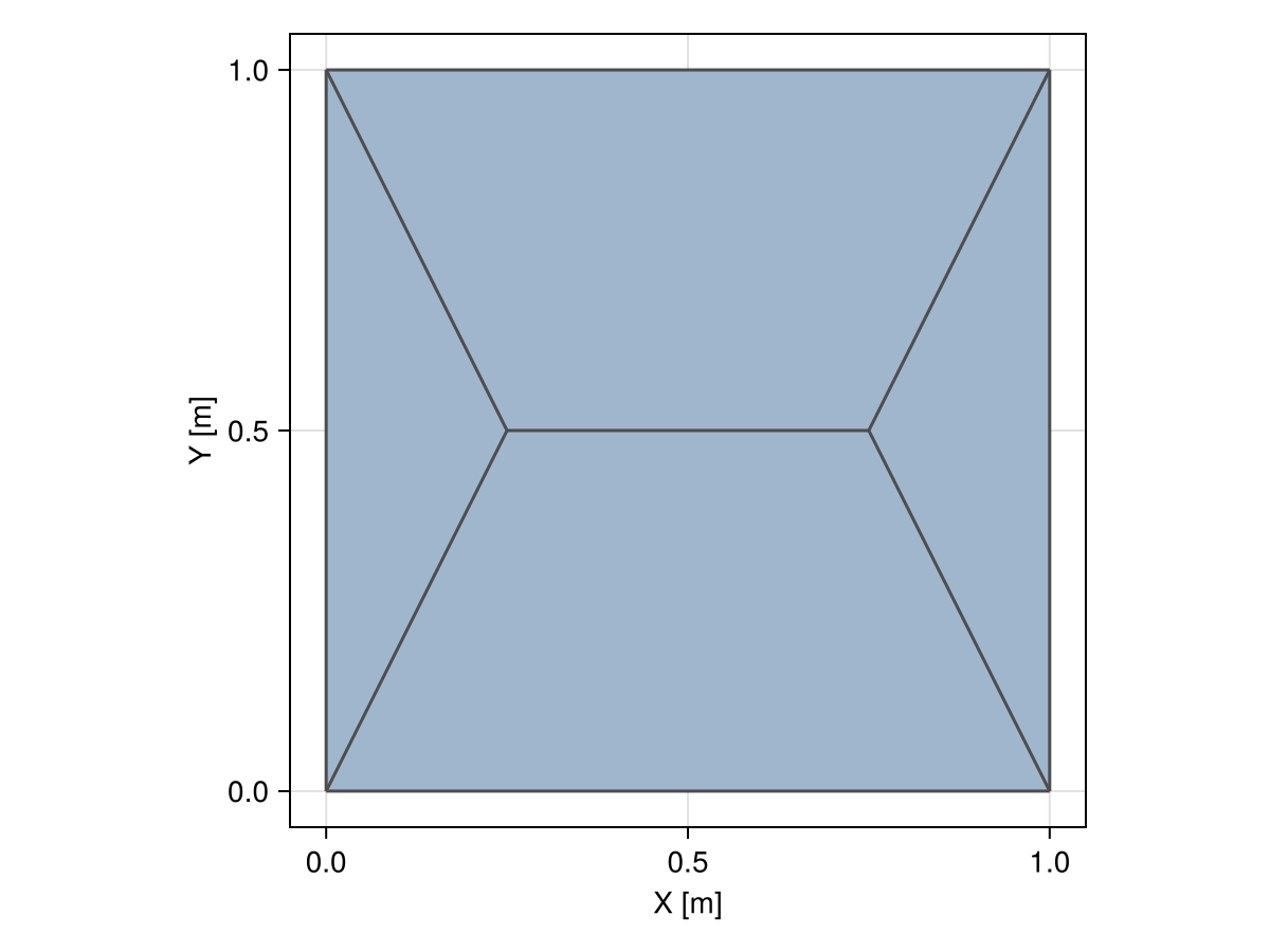

The actual geometries of the elements are materialized in a lazy fashion like with the Cartesian grid:

collect(mesh)

4-element Vector{Ngon{N, 2, Float64} where N}:
 Triangle((0.0, 0.0), (0.25, 0.5), (0.0, 1.0))
 Triangle((1.0, 1.0), (0.75, 0.5), (1.0, 0.0))
 Quadrangle((0.0, 0.0), ..., (0.25, 0.5))
 Quadrangle((1.0, 1.0), ..., (0.75, 0.5))